How to use Moment Forests on Stata
I. Components
The source code is organized into two main directories: jars and for_Stata. The most recent and actively updated files are available in the Refactor branch of the repository.
-
The
jarsfolder contains supporting Java utilities, including the compiledmomentforests.jarfile (built from the Java source code). -
The
for_Statafolder contains the Stata .ado file necessary for moment forest integration with Stata. It also contains the code to replicate the Monte Carlo exercises and the implementation of Card (1993) described in the sections below.
In addition, the java folder includes all Java source files that implement the Moment Forests framework. Within this folder, the core subdirectory contains general-purpose components applicable to a wide range of applications, while the examples subdirectory holds application-specific files.
II. How to run Moment Forests on Stata
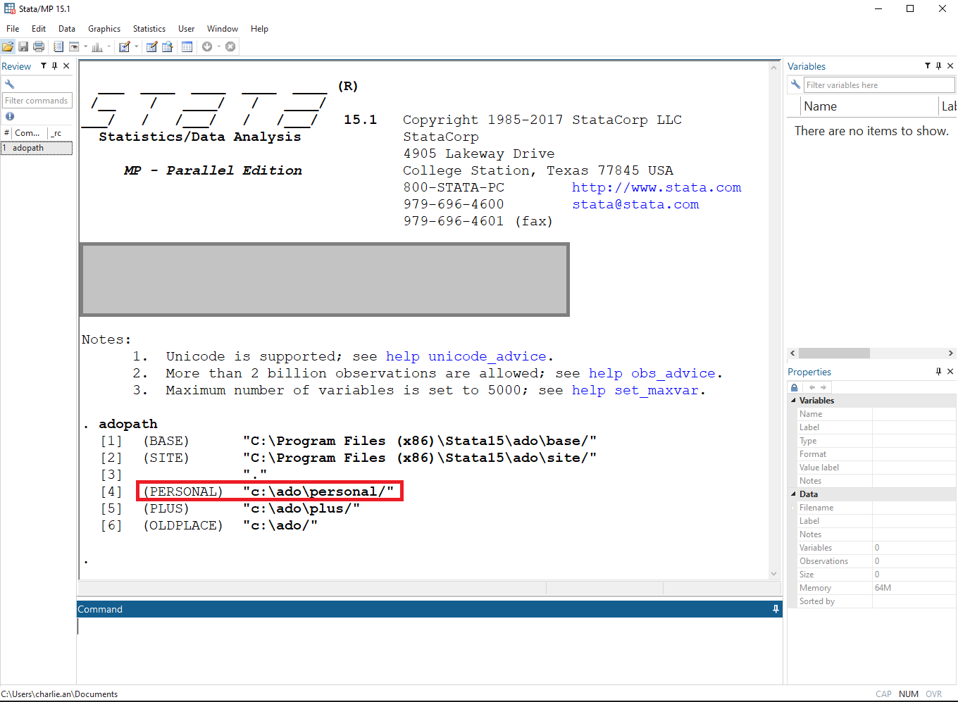
Step 1/3. Find Stata personal directory
Stata personal directory can be found by typing “adopath” in the Stata command window. The one starts with “(PERSONAL)” is the personal directory. For example, “c:\ado\personal/”.
Step 2/3. Download related files to Stata personal directory
Download the needed files to the Stata personal directory mentioned in Step 1/3.
a. .jar files
Download the .jar files from “jars” and save them in the Stata personal directory.
b. STATA files
Download the STATA .do and .ado files from “for_Stata”
Step 3/3.
Close then reopen Stata. Now you are ready to use Moment Forests on Stata!
III. Stata command “momentforest”
Variables
Y : outcome variable
X : explanatory variables that have a direct effect on the outcome variable
Z : observables that are a source of heterogeneity in the effects of X on Y
Syntax
momentforest y x [, options]
| Option | Description |
|---|---|
| Required | |
z(varlist) |
List of variables in Z. |
numtrees(integer) |
Number of trees in the moment forest. |
seed(integer) |
Random-number seed. |
| Optional | |
discretevars(varlist) |
Variables in Z that are treated as discrete. |
strata(varlist) |
One or more stratification variables in Z for stratified random sampling. |
propstructure(string) |
Proportion of observations used to estimate the structure of the trees. Default is 0.35. |
testhomogeneity(string) |
Flag for whether the moment forest should test for homogeneity. Default is true. |
cv(string) |
Flag for whether the moment forest should perform cross-validation. If cv(true) is used, you must also supply all three cvgrid() options below. |
cvgridminleaf(string) |
Space-separated values for the minimum leaf size grid (e.g., 5 10 20). Only allowed when cv(true) is set. If cv() is false, default is 25. |
cvgridminimp(string) |
Space-separated values for the minimum MSE improvement grid for a split (e.g., 0.1 1 10). Only allowed when cv(true) is set. If cv() is false, default is 0.1. |
cvgridmaxdepth(string) |
Space-separated values for the maximum tree depth grid (e.g., 3 4 5 6). Only allowed when cv(true) is set. If cv() is false, default is 5. |
gen(string) |
Stub for names of generated parameter-estimate variables. |
IV. Monte Carlo simulations
This section works through the Monte Carlo simulations in the paper. The estimator faces several simultaneous challenges: first, the moment forest has to correctly classify which components of $Z$ best improve the fit of the model without overfitting. Second, given those splits, it has to consistently estimate the parameters that best match the empirical moments. Third, it has to correctly classify and estimate parameters that are restricted to be homogeneous across the state space. Errors in one stage directly lead to errors in the other stages, so this is good test of how each of the stages of the estimator work separately and in conjunction.
The results of the simulations show the following:
- The mean-squared prediction error of the outcome variable converges rapidly in all cases to its irreducible error, suggesting that the model selection component of the estimator captures the true data-generating process very well.
- The classification rate of homogenous parameters as homogeneous is nearly 100 percent for all the replications. More importantly, the model never classifies the heterogeneous parameters as homogeneous. That matters since missing the homogeneous parameter leads to inefficiency but not bias, while incorrectly classifying the heterogeneous parameter does.
The file Monte Carlo.do in the for_Stata directory contains the code necessary to perform these Monte Carlo simulations and replicate the figures in the paper.
Linear model
Consider the following linear model:
\[Y = X'\beta(Z) + \epsilon.\]Let $X =$ { $X_1, X_2$ }, where $X_1$ is a vector of ones, $X_2 \sim N(0,2)$, and $\epsilon$ is an idiosyncratic error term that is distributed as a standard normal. Let $Z =$ { $Z_1, Z_2, Z_3$ }, with $Z_1 \sim N(0,1)$, $Z_2 \sim U[0,1]$, and $Z_3$ is a discrete variable taking on two values (1,2) with probability (0.3,0.7). There are four sample sizes, $n \in$ { $500, 1000, 2000, 4000$ }, and three different $\beta(Z)$ corresponding to the cases of no parameter heterogeneity, heterogeneity in only one dimension of $X$, and heterogeneity in both dimensions of $X$. For each configuration, the code contrast the performance of the estimator against the unrestricted model where no parameters are identified as being universally homogeneous. Each Monte Carlo experiment is repeated 500 times to obtain distributions of the statistics of interest.
To test these three stages, we simulate three scenarios. First, we consider a fully heterogeneous parameter specification:
\[\beta(Z) = \begin{cases} (-1.0, 1.0) & \text{ if } Z_1 > 0 \\ (0.33, -1.0) & \text{ else.} \end{cases}\]In the second scenario, we restrict one of the parameters to be homogeneous across the state space:
\[\beta(Z) = \begin{cases} (-1.0, 1.0) & \text{ if } Z_1 > 0 \\ (-1.0, -1.0) & \text{ else.} \end{cases}\]And in the third case, we fix parameters to be homogeneous everywhere:
\[\beta(Z) = (-1.0, 1.0).\]Partially linear model
Next, consider a more complex model where one of the components is infinite-dimensional. The challenge here is to ensure that the estimator continues to classify the components appropriately and to see how well it can do in approximating the infinite-dimensional part. The data-generating process is more involved:
\[Y = \beta_1(Z) + \beta_2 X_2,\]with $\beta_1(Z) = 2.5 \sin{Z} + 0.25 Z^2$ and $\beta_2=1.0$.
V. Worked example - Card (1993)
To further illustrate the model, this section revisit the classic study of Card (1993), which investigates the relationship between schooling and income. He uses two empirical techniques with a variety of parametric specifications: a baseline assessment of correlations using ordinary least squares (OLS) and a causal estimate using instrumental variables. The OLS estimates, controlling for a variety of demographic variables and fixed effects, show that higher levels of education are correlated with higher wages. The study is typical of most, if not all, empirical papers, in that Card conducts “robustness checks” by reporting results under various (ad hoc) parametric specifications. Further, the issue of finding the correct specification, particularly with regard to observable heterogeneity in the relationship between wages and education across different subgroups, is a first-order concern in this literature. In his landmark overview of the literature on education and wages in the Handbook of Labor Economics, Card (1999) poses two critical and interrelated issues: What functional form should the wage regression take and how should it vary across different subgroups? This estimator is designed to answer these types of questions.
Card (1993) utilizes data from the National Longitudinal Survey of Young Men (NLSYM), a panel dataset tracking men aged 14 to 24 from 1966 to 1981. The NLSYM provides information on educational attainment, wages, work experience, and the socioeconomic background of the respondents. It also includes geographic variables, specifying the region of the United States where the respondent has resided, whether they have lived in a Standard Metropolitan Statistical Area (SMSA), and local labor market conditions. The outcome variable is the log of hourly wages in 1976, and the primary explanatory variable of interest is total years of schooling. Control variables include work experience and socioeconomic and regional indicators. In particular, years of parental education are used as proxies for the respondent’s family background.
Revisiting Card (1993) using moment forests provides a more flexible and data-driven approach to estimating the returns to education, addressing some of the limitations in the methods used in the original paper. For one, while Card had to hypothesize at the beginning of the analysis that returns to education varied by parental background, moment forests allow us to detect heterogeneous effects without any presuppositions. Instead, the moment forest employs a data-driven approach to determine heterogeneity. Additionally, the traditional approach to working with regressions relies on multiple model specifications to perform robustness checks on the results. This approach is both ad hoc and prone to researcher discretions. Moment forests mitigate this issue by finding the best specification within the class of linear models. Moreover, they provide semiparametric estimation that can capture nonlinearity in the relationships of the variables.
The file CardStata dofile.do in the for_Stata directory contains the code necessary to perform these Monte Carlo simulations and replicate the figures in the paper.
Consider the empirical specification given by
\[Y = X'\beta(Z) + \epsilon\]Here, $X$ contains the explanatory variables that have a direct effect on the outcome $Y$, and $Z$ consists of the observables that are a source of heterogeneity in the effects of $X$ on $Y$. Moment forests bring two important innovations to Card’s process. First, the moment forest can identify which variables exhibit heterogeneity. The Holm-Bonferroni procedure is used to determine which variables in $X$ are homogeneous and which are heterogeneous. Second, rather than testing multiple specifications, the moment forest directly identifies the most relevant variables. The variables in $Z$ that the forest selects for splitting are the ones pertinent for analysis. In this application, we find the best specification among the models of the form given by the equation above. In other words, we find the simplest model that is not statistically rejected by the data. To accomplish this, we perform an iterative analysis using moment forests. We begin with the most flexible model and add variables into $X$ based on the splitting behavior of the forest. This process terminates when the moment forest no longer makes any splits. At that point, the forest will have captured all the observable heterogeneity in the data.
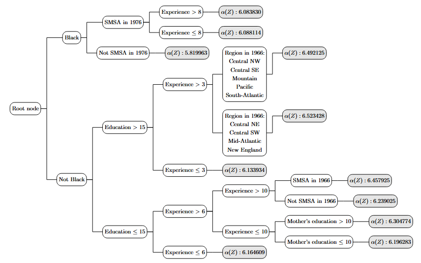
We begin our analysis with a purely descriptive exercise. We set the moment function to be just the constant, which generates the classic regression tree:
\[m(X;\beta(Z)) = \alpha(Z).\]We start with this specification as it allows for model-free exploration of the data. This model is a universal approximator, so we are not imposing any restrictions on the underlying DGP by using just a constant. The patterns that this specification reveals can be useful in guiding further exploration. The moment forest split on the respondent’s years of education, work experience, and living region in almost all of its trees, and it split on the indicator for Black in 70% of them. This suggests that these variables are highly correlated with hourly wages. In addition, the moment forest split on the father’s and mother’s years of education in 32% and 60% of the 50 trees respectively. This is in line with Card’s supposition that parental education levels can affect children’s future earnings. The figure below plots the first regression tree in the forest with CV parameters on OLS. It shows that Black respondents received lower wages than White respondents. Average hourly wages varied significantly for White respondents but were all higher than those of Black respondents.
The moment forest split on education in all but one of it’s trees. This is reassuring, as it shows that years of schooling is strongly related to earnings. If the moment forest did not split on our primary explanatory variable of interest, our analysis would already be finished. In the next exercise, we include both a constant and years of education in $X$:
\[m(X;\beta(Z)) = \alpha(Z) + \beta(Z)\cdot education\]We find that $\alpha(Z)$ was overwhelmingly voted as heterogeneous across the trees in the forest. Education was heterogeneous in 60\% of the trees and hence determined to be heterogeneous in the moment forest. This suggests that the returns to education varied across subgroups in the data. The following figure plots the first tree in the moment forest.
The objective of these first exercises is to search for patterns in the data and help determine which variables should be interest. It also finds observable heterogeneity in the reduced form and sets the stage for further data exploration and analysis. The moment forest split on years of worked experience and living region in 1966 in all of its trees. This suggests that those have important correlation with earnings. Therefore, we next implement a moment forest with those variables in the $X$ matrix. Note that although some categorical variables are frequently split on in the moment forest, we don’t need to include them in $X$. This is because they are just nuisance parameters and will be captured in splits on the constant.
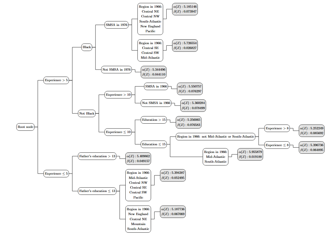
First, we add years of work experience into $X$:
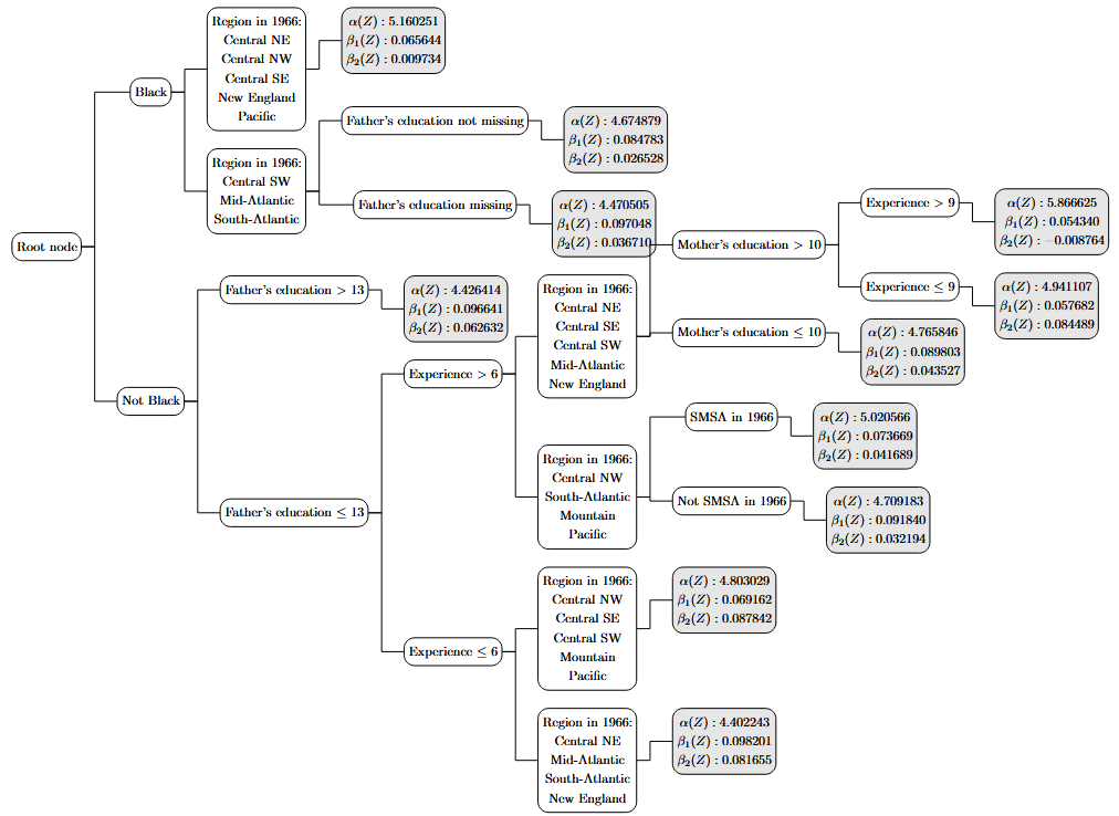
\[m(X;\beta(Z)) = \alpha(Z) + \beta_1(Z)\cdot education + \beta_2(Z)\cdot experience\]We find that $\alpha(Z)$ was determined to be heterogeneous in 90% of the trees in the forest and $\beta_2(Z)$ was heterogeneous in all of them. $\beta_1(Z)$ was also heterogeneous but only so in 60% of the trees. This suggests that subgroups in the data had different mean hourly wages and returns to both education and work experience. The plot of the first tree shows that Black respondents generally had lower hourly wages and received lower returns, especially in work experience. It also demonstrates a large degree of heterogeneity in returns to education and work experience across parental education levels. Black respondents living in the Atlantic or Central South West regions differed by whether their father’s level of education was missing or not. For White respondents, the returns to schooling were heterogeneous across both parents’ levels of education.
Next, we add a categorical variable for living region in 1966 in $X$. This is because, as shown in the third column of Table~\ref{tab:moment forest splitting criteron}, the prior moment forest split on this variable in all but one of it’s trees.
\[m(X;\beta(Z)) = \alpha(Z) + \beta_1(Z)\cdot education + \beta_2(Z)\cdot experience + \sum\limits_{r=1}^{8} \delta_r(Z) \cdot 1\{region\_1966 = r\}\]where $\delta_r(Z)$ represents the set of fixed effects for living region in 1966 with region $r=9$, the Pacific, omitted. $\beta_2(Z)$ was voted as heterogeneous, but all the other parameters were determined to be homogeneous. It estimated a value for the constant of $\alpha = 4.240$ and a homogeneous value to the returns to education at $\beta_1 = 0.095$. The results show that the variables that the forest is still splitting on geographic indicator variables. This motivates that there may be interaction effects between the heterogeneous work experience and living region. As such, we add interaction terms between work experience and living region in 1966 in $X$:
\[m(X;\beta(Z)) = \alpha(Z) + \beta_1(Z)\cdot educ + \beta_2(Z)\cdot exp + \sum\limits_{r=1}^{8}\left( \delta_r(Z) + \gamma_r(Z)\cdot exp\right)\cdot 1\{reg\_1966 = r\}\]where $\alpha(Z)$ represents possible group-specific intercepts, $\delta_r(Z)$ represent the set of fixed effects for living region in 1966, and $\gamma_r(Z)$ represent the set of fixed effects for the interaction between work experience and living region in 1966. The forest finds that all the parameters are homogeneous and does not make any splits. Hence, we determine that this moment specification is our “final” specification and we terminate our iterative process.
Our methodology reveals that the true linear specification for estimating a respondent’s log earnings is to use years of education and work experience as explanatory variables and to include fixed effects for living region in 1966 and the interaction between work experience and living region in 1966. This specification has some important differences from the ones considered in Card (1993). Notably, we do not find any nonlinearity in the returns to years of work experience. Furthermore, we do not find any evidence that parental education affects the returns to education. While prior forests split on variables such as parental education and race indicators, the final specification suggests that what those forests perceived to be heterogeneity were captured by geographic differences.