Worked Examples of Moment Forests

I. Data Generation Process

In order to show the overall performance of the algorithm, we proceeded with three simulations based on different types of parameters.

\[ Y = W \beta + \epsilon \] where \( W \) is a treatment dummy variable and \( \epsilon \) follows N(0,1)

1. discrete case: \( \beta(x1,x2) = x1 +10*(x2 -1) \), where \( x1, x2 = {1,..,10} \)
2. continuous case: \( \beta(x) = sin(x) \), where \( x = (0,2 \pi) \)
3. hybrid case: \( \beta(x1,x2) = sin(x1)*(x2 -5) \), where \( x1= (0,2 \pi) \) & \( x2 = {1,..,10} \)

II. Monte Carlo Simulation

Step 1/4. Download the simulation datasets and Stata do file in here to your own working directory.

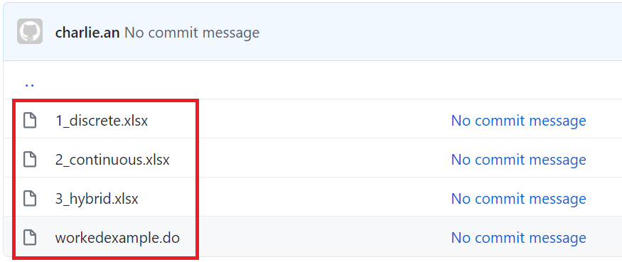
Step 2/4. Open Stata and open the Stata do file downloaded (workedexample.do).

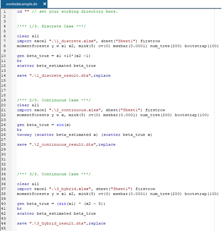
Step 3/4. Set your working directory in the do file.

For example, cd "C:\Users\Valued Customer"

Step 4/4. Run the code.

III. Simulation Results

The estimation results are reported and plotted below.

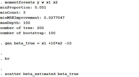
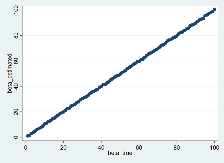
1/3. Discrete Case: \( \beta(x1,x2) = x1 +10*(x2 -1) \)

Results printed on Stata window

Scatter plot, true beta against estimated beta

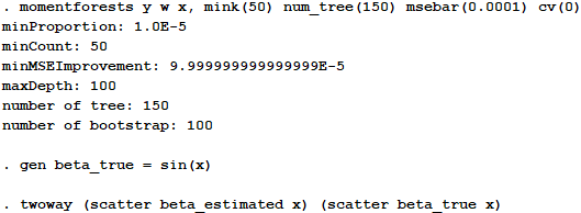
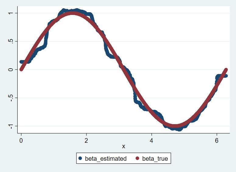
2/3. Continuous Case: \( \beta(x) = sin(x) \)

Results printed on Stata window

Scatter plot, x against estimated beta

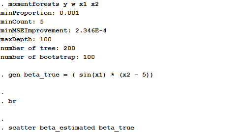
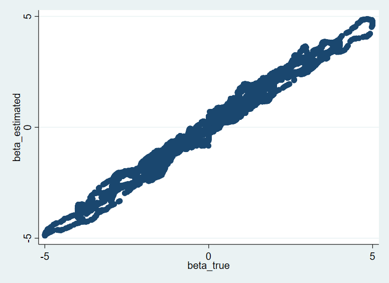
3/3. Hybrid Case: \( \beta(x1,x2) = sin(x1)*(x2 -5) \)

Results printed on Stata window

Scatter plot, true beta against estimated beta

back